Introduction to Gaussian Processes for Time Dependent Data

Virginia Tech

Parul Vijay Patil, Leah R. Johnson, Robert B. Gramacy

Outline

We will go through the following topics:

1. Motivation as Ecologists

2. Introducing Gaussian Processes (GPs)

3. Hyper-Parameters in GPs

4. Fitting a GP with some code

5. Heteroskedastic GPs (HetGPs)

6. Fitting a HetGP with some code

7. Motivating Ecological Example: Hands-On Practice

Time-Depedent Data

• In ecology, we often have data with features such as:

  • Sparse and irregularly sampled time series (Time-Dependent Data).

  • Varies from location to location.

  • Often consists of several noisy observations due to sampling errors.

Gaussian Process: Introduction

• Gaussian Process (GP) models are non paramteric and flexible regression model.

• Excellent for uncertainty quantification (UQ).

• Suppose we have n observations Y_n corresponding to X_n inputs, then

Y_{n} \sim N (\mu, \Sigma_n)

• We wish to estimate the response at a new input X_p i.e. Y_p \mid Y_n, X_n.

• Note: If you set \mu = X \beta and \Sigma_n = \sigma^2 \mathbb{I}, we have a Linear Regression (LR) Setup.

Distance

• For a GP, the covariance matrix, \Sigma_n is defined by a distance based kernel.

• Consider,

\Sigma_n = \tau^2 C_n \quad \text{where} \quad C_n^{ij} = \exp \left( - \vert \vert x_i - x_j \vert \vert^2 \right)

• The covariance structure now depends on how close together the inputs.

• The covariance will decay at an exponential rate as x moves away from x'.

Visualizing a GP

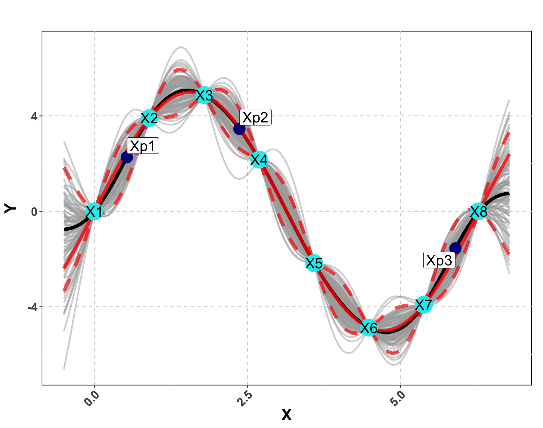
Predictions using the Data

• We wish to find \mathcal{Y} \vert X_n, Y_n and we know Y_n \vert X_n \sim \mathcal{N}( 0, \Sigma_n).

• First we will “stack” the predictions and the data.

\begin{equation*} \begin{bmatrix} \mathcal{Y} \\ Y_n \\ \end{bmatrix} \ \sim \ \mathcal{N} \left( \; \begin{bmatrix} 0 \\ 0 \\ \end{bmatrix}\; , \; \begin{bmatrix} \Sigma(\mathcal{X}, \mathcal{X}) & \Sigma(\mathcal{X}, X_n)\\ \Sigma({X_n, \mathcal{X}}) & \Sigma_n\\ \end{bmatrix} \; \right) \end{equation*}

• By properties of Normal distribution, \mathcal{Y} \vert X_n, Y_n is also normally distributed.

• We can notate this as:

\begin{equation*} \begin{aligned} \mathcal{Y} \mid Y_n, X_n \sim \mathcal{N} \left(\mu(\mathcal{X}), \sigma^2(\mathcal{X})\right) \end{aligned} \end{equation*}

Distribution of Interest!

• We will apply the properties of conditional Normal distributions.

\begin{equation*} \begin{aligned} \mu(\mathcal{X}) & = \Sigma(\mathcal{X}, X_n) \Sigma_n^{-1} Y_n \\[10pt] \sigma^2(\mathcal{X}) & = \Sigma(\mathcal{X}, \mathcal{X}) - \Sigma(\mathcal{X}, X_n) \Sigma_n^{-1} \Sigma(X_n, \mathcal{X}) \\ \end{aligned} \end{equation*}

• To make predictions at a single new location x, \Sigma(x, x) = 1 + g.

• We need to focus on \Sigma so we can tune our GP appropriately.

Sigma Matrix

• \Sigma_n = \tau^2 \left( C_{\theta}(X_n) + g \mathbb{I_n} \right) where C_n is our kernel.

• One of the most common kernels which we will focus on is the squared exponential distance kernel written as

C_\theta(x, x') = \exp{ \left( -\frac{\vert\vert x - x' \vert \vert ^2}{\theta} \right ) }

• What’s \tau^2, g and \theta though? No more math. We will just conceptually go through these

Hyper Parameters

A GP is non parameteric, however, has some hyper-parameters. In this case,

• \tau^2 (Scale): This parameter can be used to adjust the amplitude of the data.

• \theta (Length-scale): This parameter controls the rate of decay of correlation.

• g (Nugget): This parameter controls the noise in the covariance structure (adds discontinuity)

These hyper-parameters \{ \tau^2, \theta, g \} are inferred using MLE/Bayesian schemes.

Scale (Amplitude)

• A random draw from a multivariate normal distribution with \tau^2 = 1 will produce data between -2 and 2.

• Now let’s visualize what happens when we increase \tau^2 to 25.

Length-scale (Rate of decay of correlation)

• Determines how “wiggly” a function is

• Smaller \theta means wigglier functions i.e. visually:

Nugget (Noise)

• Ensures discontinuity and prevents interpolation which in turn yields better UQ.

• We will compare a sample from g ~ 0 (< 1e-8 for numeric stability) vs g = 0.1 to observe what actually happens.

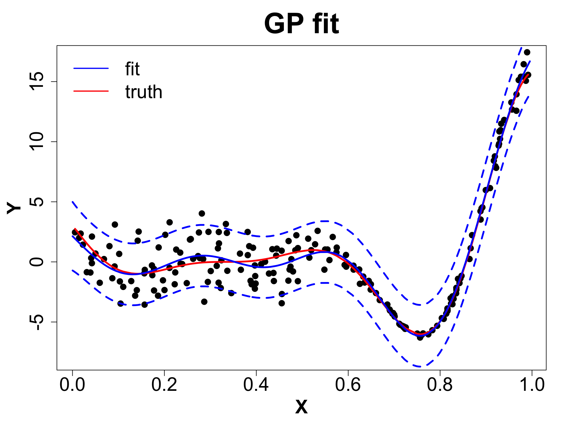
Toy Example (1D Example)

X <- matrix(seq(0, 2*pi, length = 100), ncol =1)
n <- nrow(X) 
true_y <- 5 * sin(X)
obs_y <- true_y + rnorm(n, sd=1)

XX <- matrix(seq(0, 2*pi, length = 200), ncol =1)

Toy Example (1D Example)

eps <- sqrt(.Machine$double.eps)

# Fit GP
gpi <- newGP(X = X, Z = obs_y, d = 0.1, 
        g = 0.1 * var(obs_y), dK = TRUE)

# Obtain MLE
mle <- mleGP(gpi = gpi, param = c("d", "g"),
        tmin= c(eps, eps), tmax= c(10, var(obs_y)))

# Make Predictions
p <- predGP(gpi = gpi, XX = XX)

Toy Example (1D Example)

eps <- sqrt(.Machine$double.eps)

# Fit GP
gpi <- newGP(X = X, Z = obs_y, d = 0.1, 
        g = 0.1 * var(obs_y), dK = TRUE)

# Obtain MLE
mle <- mleGP(gpi = gpi, param = c("d", "g"),
        tmin= c(eps, eps), tmax= c(10, var(obs_y)))

# Make Predictions
p <- predGP(gpi = gpi, XX = XX)

mean_gp <- p$mean
s2_gp <- diag(p$Sigma)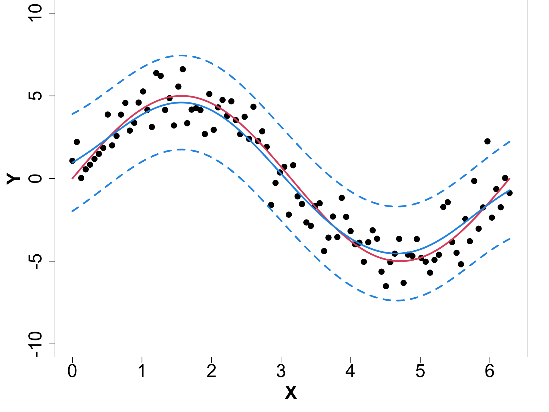

Extentions: Anisotropic Gaussian Processes

• Suppose we have a d dimensional input space, X_{n \times d}. We can have one length-scale for each dimension i.e. \mathbf{\theta} = \{ \theta_1, \dots, \theta_d \}.

• In this situation, we can rewrite the C_n matrix as,

C_\theta(x , x') = \exp{ \left( -\sum_{k=1}^{d} \frac{ (x_k - x_k')^2 }{\theta_k} \right )}

• This is also called a Seperable GP

• We will explore newGPsep, mleGPsep and predGPsep.

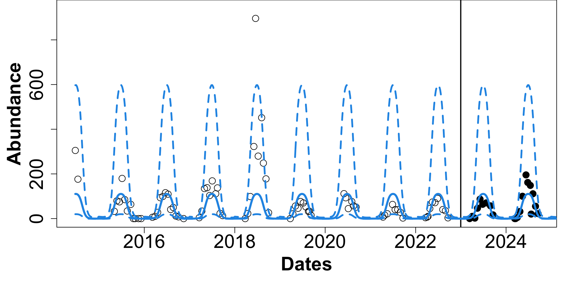
Tick Populations: ORNL

	Iso-week (c)	Periodicity	Transformed Density
2014-06-23	0.49	1.00	5.72
2014-07-14	0.55	0.98	5.18
2015-05-04	0.36	0.82	3.51

# Fitting the GP
gpi <- newGPsep(X, y, d = 0.1, 
          g = 0.1 * var(y), dK = T)

# Calculating MLEs jointly
mle <- mleGPsep(gpi)

# Predictions
ppt <- predGPsep(gpi, XXt)

Tick Populations: ORNL

	Iso-week (c)	Periodicity	Transformed Density
2014-06-23	0.49	1.00	5.72
2014-07-14	0.55	0.98	5.18
2015-05-04	0.36	0.82	3.51

# Fitting the GP
#| code-line-numbers: "|9|"
gpi <- newGPsep(X, y, d = 0.1, 
          g = 0.1 * var(y), dK = T)

# Calculating MLEs jointly
mle <- mleGPsep(gpi)

# Predictions
ppt <- predGPsep(gpi, XXt)

Extension: Heteroskedastic GPs (HetGP)

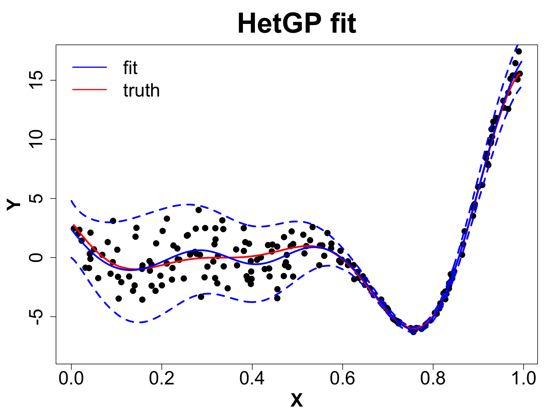
• Suppose we have noise is input dependent (Binois, Gramacy, and Ludkovski 2018).

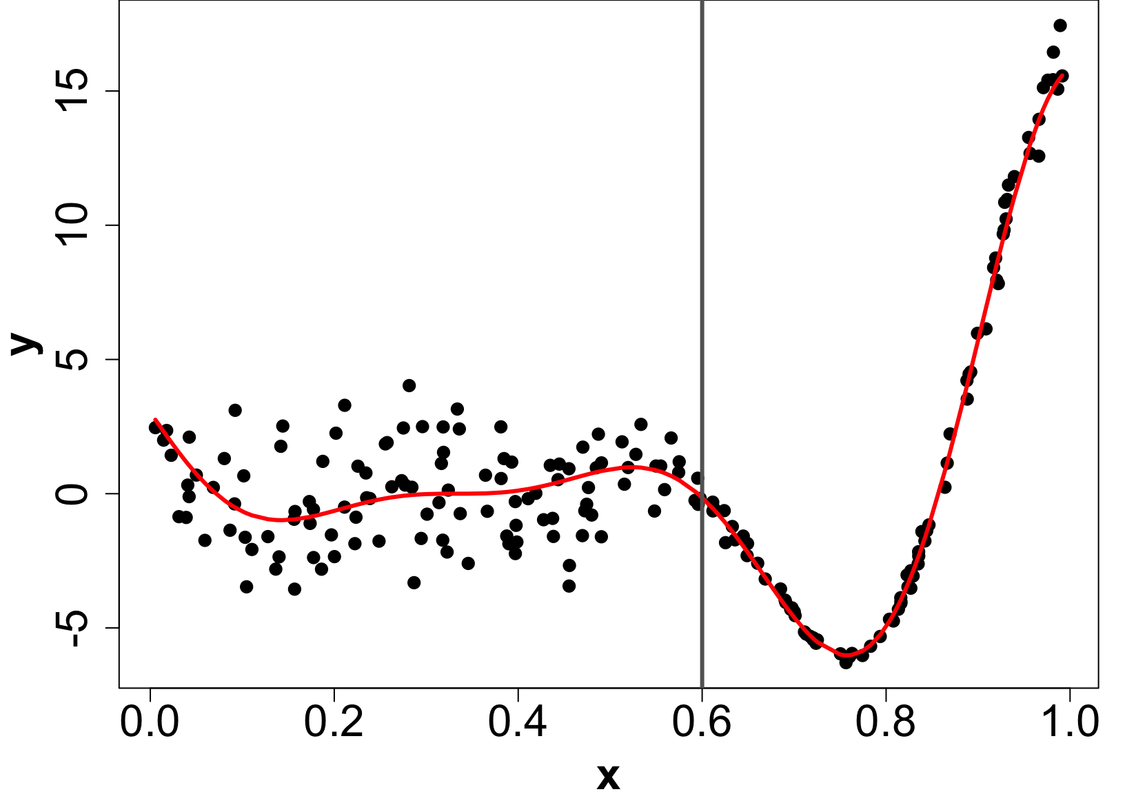
Extension: Heteroskedastic GPs (HetGP)

• Suppose we have noise is input dependent (Binois, Gramacy, and Ludkovski 2018).

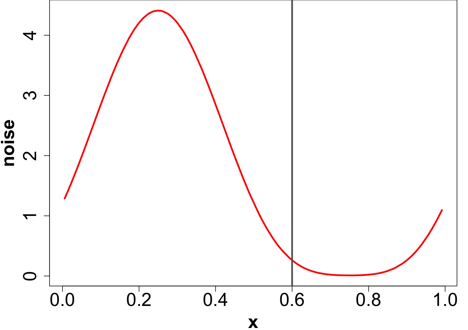
• We can use a different nugget for each unique input rather than a scalar g.

HetGP Setup

• Let X_n, Y_n be the data and \mathbf{\lambda_n} be the noise level at input X_n.

• In case of a hetGP, we have:

\begin{align*} Y_n & \sim GP \left( 0, \tau^2 \left( C_{\theta_Y}(X_n) + \Lambda_n \right) \right) \quad \text{where,} \quad \Lambda_n = \text{Diag}(\bold{\lambda}_n);\\ \log \bold{\lambda}_n & \sim GP \left( 0, \tau_\lambda^2 C_{\theta_\lambda}(X_n) \right)\\ \end{align*}

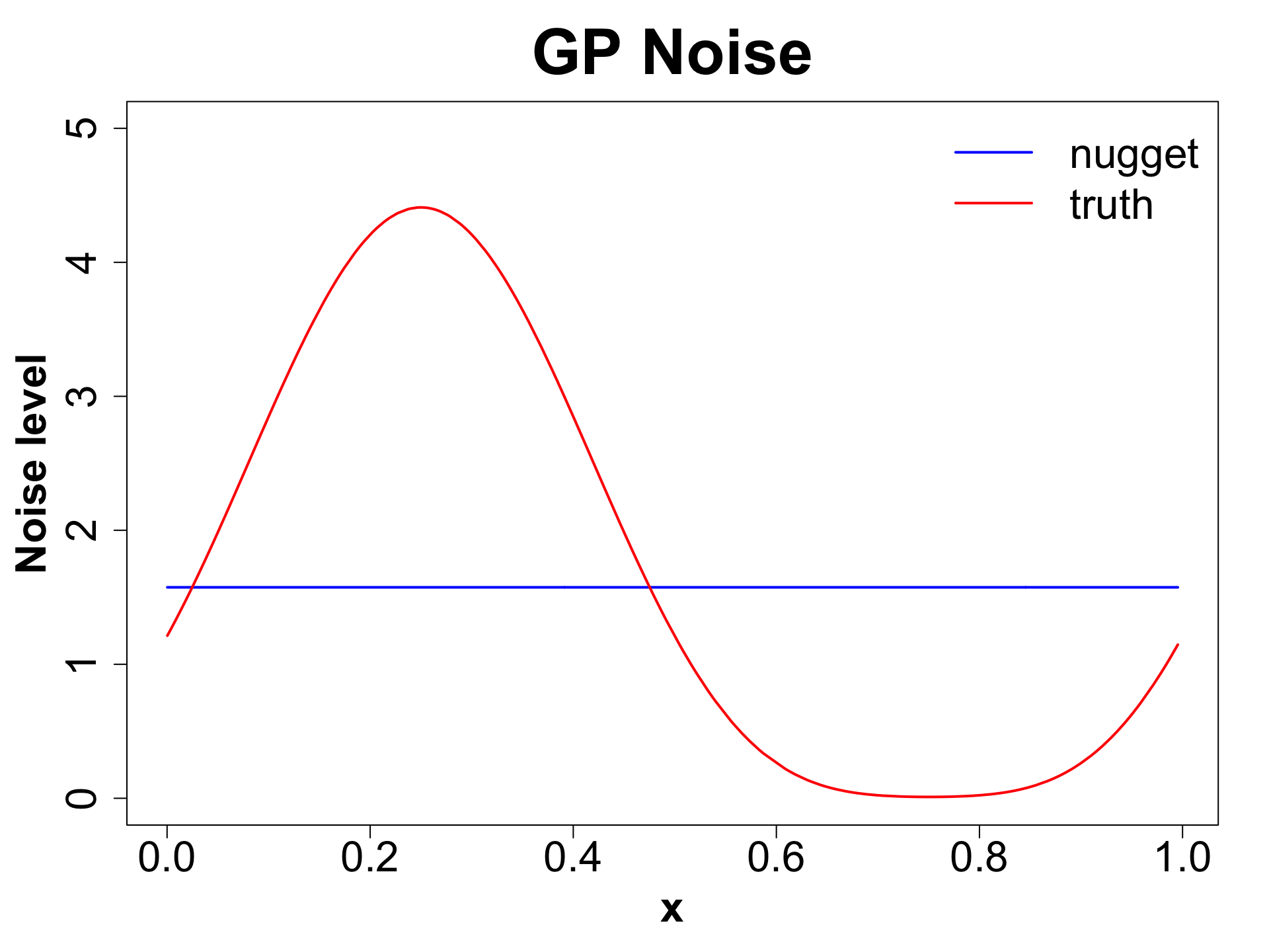
• Note that in a regular GP: \Lambda_n = g \mathbb{I}_n. We average over the noise across the input space.

• We must infer \{ \bold{\lambda}_n, \theta_Y, \theta_\lambda, \tau^2, \tau^2_\lambda \} using MLE/Bayesian schemes.

HetGP Predictions

• For a new location \mathcal{X}, we use \Sigma_n = \tau^2 (C_{\theta_Y} (X_n) + \Lambda_n).

\begin{aligned} \mu(\mathcal{X}) & = \Sigma(\mathcal{X}, X_n) \Sigma_n^{-1} Y_n \\ \sigma^2(\mathcal{X}) & = \tau^2 [1 + \lambda(\mathcal{X})] - \Sigma(\mathcal{X}, X_n) \Sigma_n^{-1} \Sigma(X_n, \mathcal{X}) \\ \end{aligned}

• How do we infer \lambda(\mathcal{X})?

• Plug in \Sigma_n^{(\lambda)} = \tau_\lambda^2 C_{\theta_\lambda}(X_n) and Y_n = \bold{\lambda}_n in the GP predictive equations. Why?

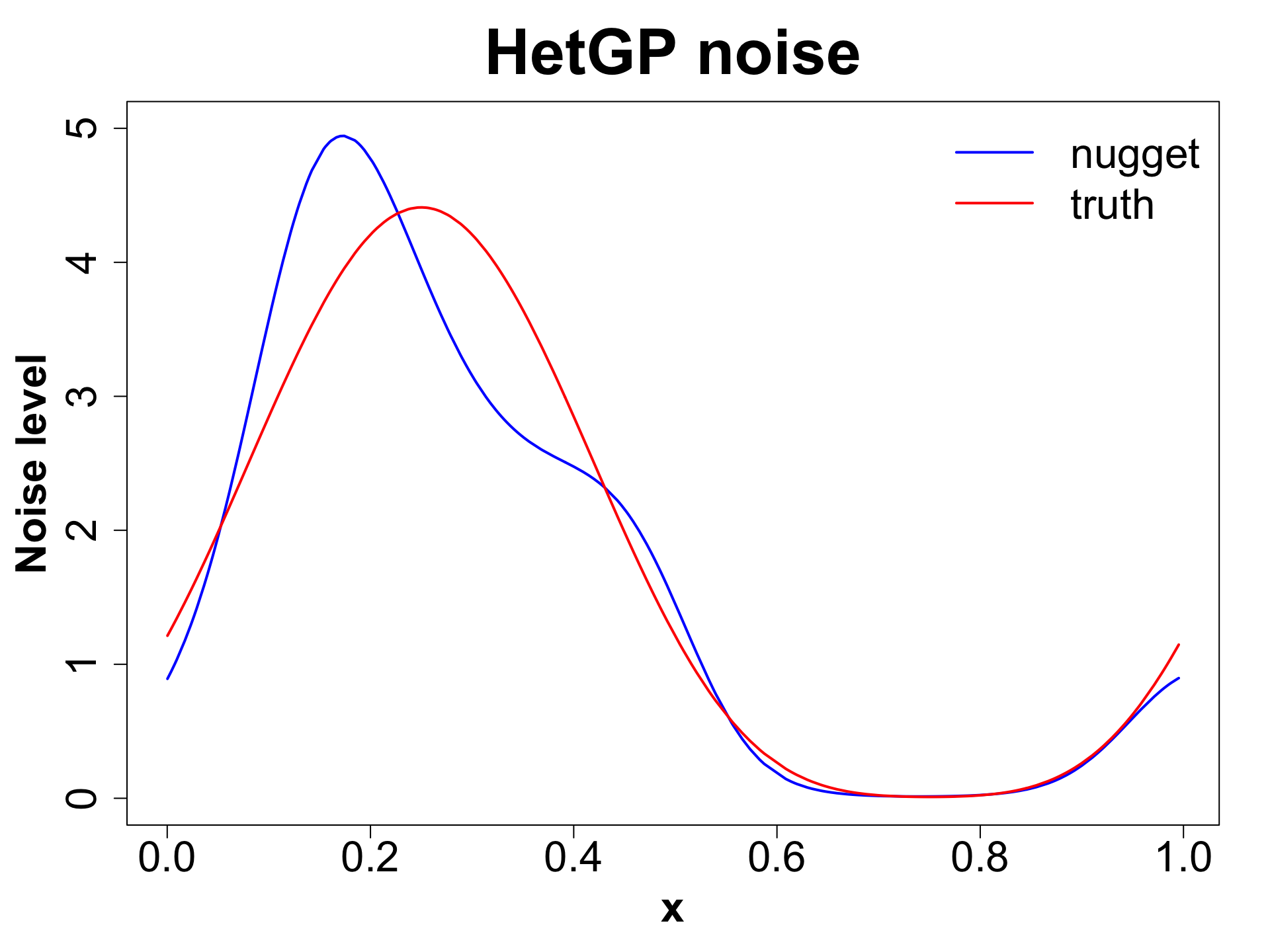
• Obtain \mu_\lambda(\mathcal{X}) and \sigma^2_\lambda(\mathcal{X}). Use \mu_\lambda(\mathcal{X}) as estimated noise level \lambda(\mathcal{X}).

HetGP: Toy Example (1D Example)

homgp <- mleHomGP(x, y)
p_hom <- predict(object = homgp, x = XX)

mean_gp <- p_hom$mean
s2_gp <- p_hom$sd2 + p_hom$nugs

HetGP: Toy Example (1D Example)

homgp <- mleHomGP(x, y)
p_hom <- predict(object = homgp, x = XX)

mean_gp <- p_hom$mean
s2_gp <- p_hom$sd2 + p_hom$nugs

hetgp <- mleHetGP(x, y)
p_het <- predict(object = hetgp, x = XX)

mean <-  p_het$mean
s2 <-  p_het$sd2 + p_het$nugs

HetGP: Noise Levels

Tick Population Forecasting

• EFI-RCN held an ecological forecasting challenge NEON Forecasting Challenge (Thomas et al. 2022)

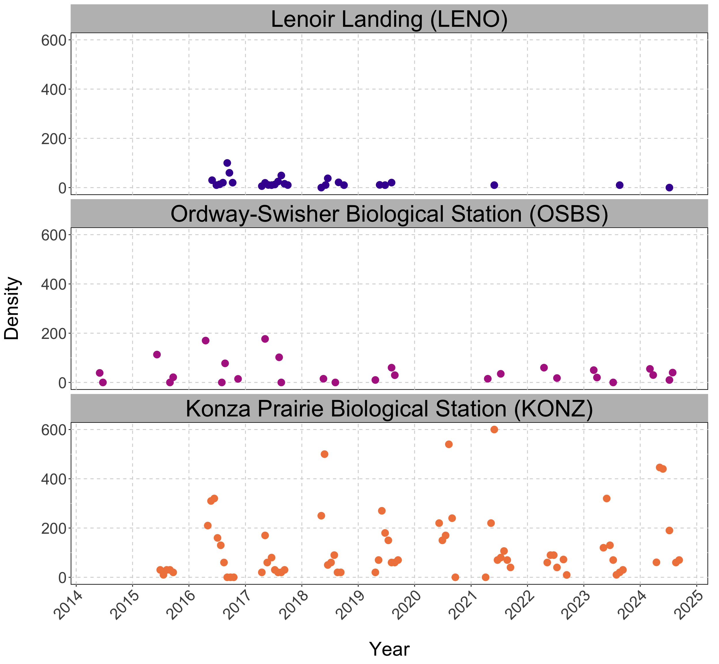
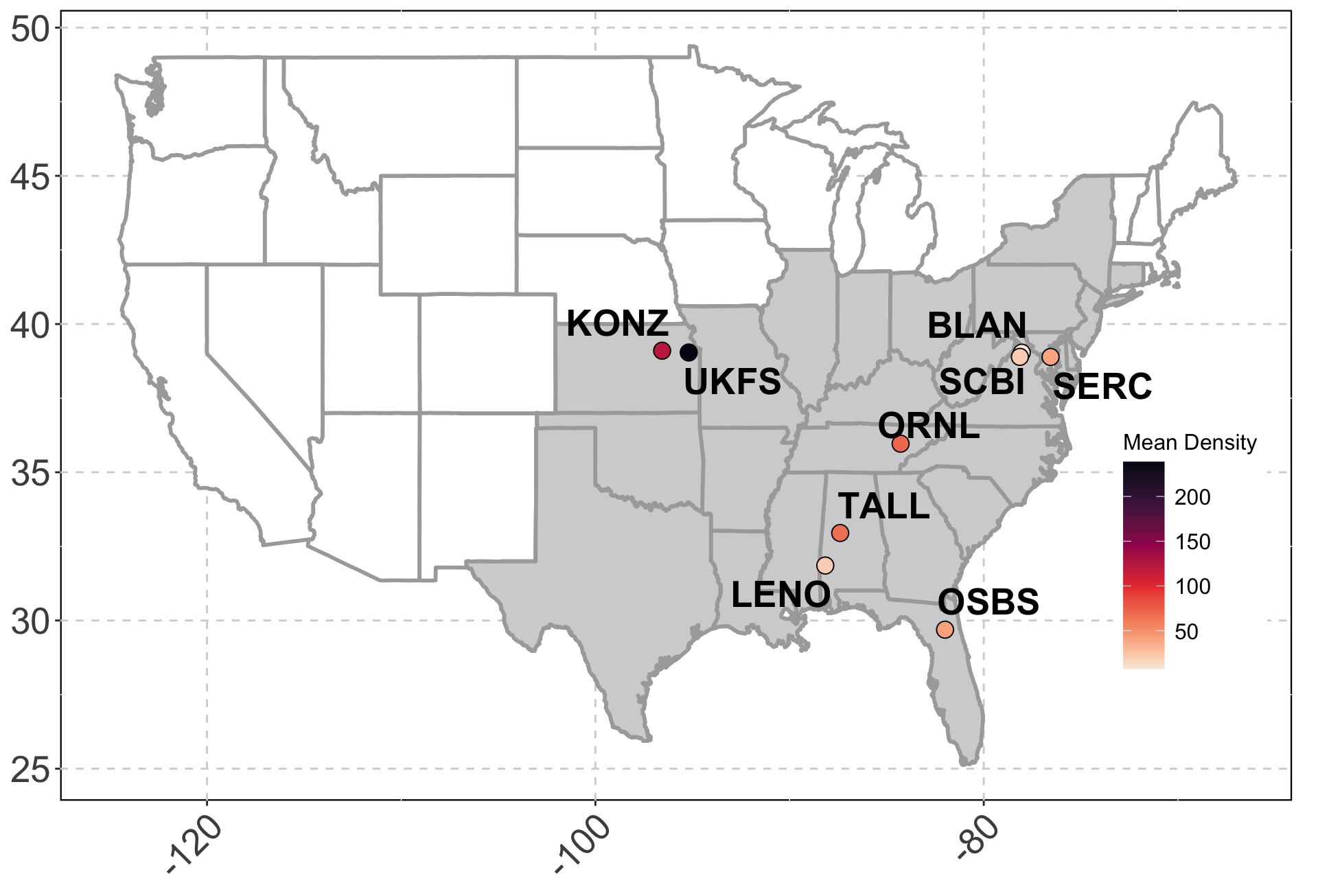
• We focus on the Tick Populations theme which studies the abundance of the lone star tick (Amblyomma americanum)

• Objective: Forecast tick density for 4 weeks into the future.

• Sites: The data is collected across 9 different NEON plots.

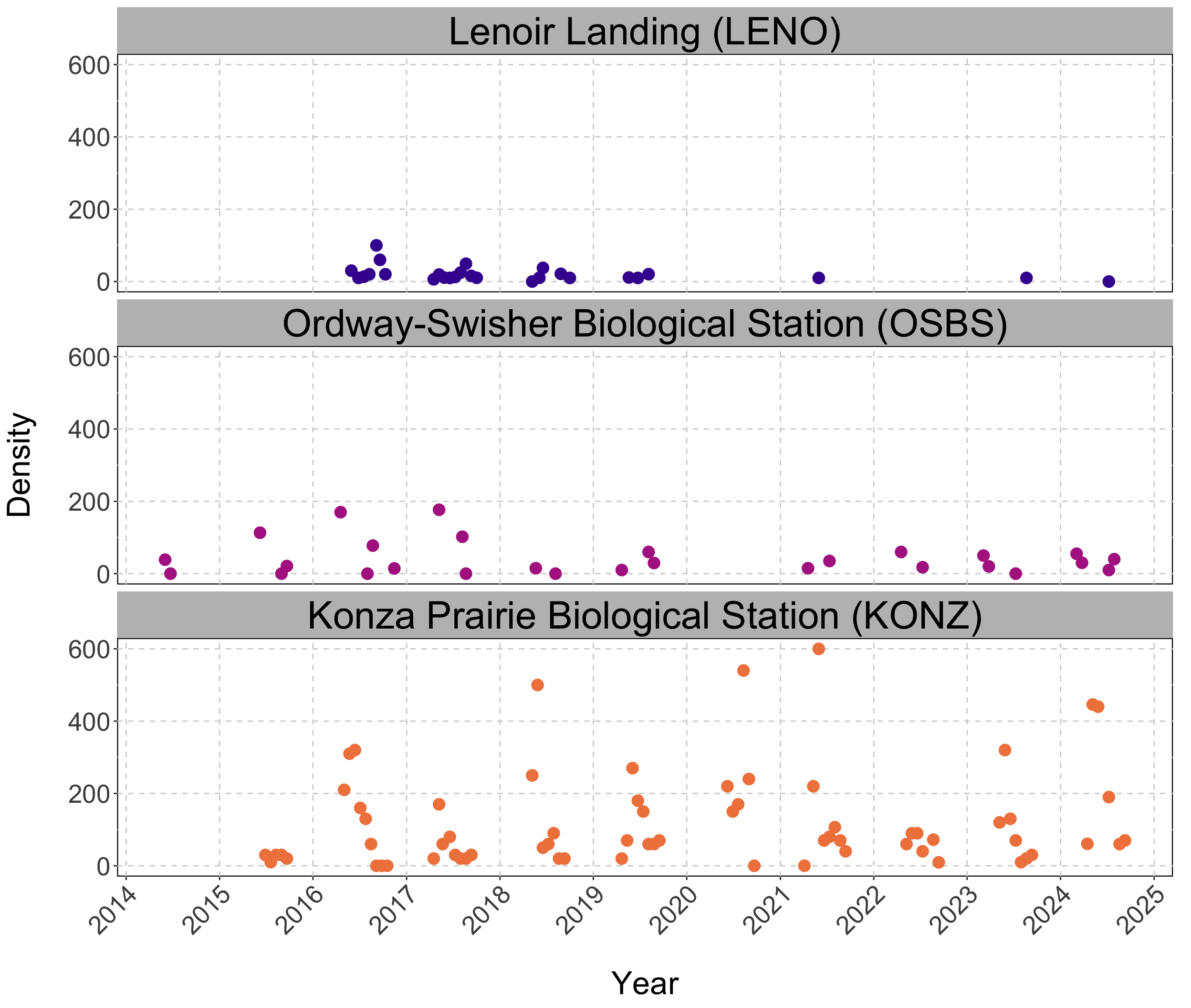
• Data: Sparse and irregularly spaced.

• n = ~570 observations since 2014.

Predictors

• Iso-week, X_1 = 1,2,... 53.

• Periodicity, X_2 = \text{sin}^2 \left( \frac{2 \pi X_1}{106} \right).

• Mean Elevation, X_3.

Practical

• Setup these predictors
• Transform the data to normal
• Fit a GP to the Data
• Make Predictions on a testing set
• Check how predictions perform.

References

Binois, Mickael, Robert B Gramacy, and Mike Ludkovski. 2018. “Practical Heteroscedastic Gaussian Process Modeling for Large Simulation Experiments.” Journal of Computational and Graphical Statistics 27 (4): 808–21.

Thomas, R Quinn, Carl Boettiger, Cayelan C Carey, Michael C Dietze, Leah R Johnson, Melissa A Kenney, Jason S Mclachlan, et al. 2022. “The NEON Ecological Forecasting Challenge.” Authorea Preprints.